Friday, January 13, 2012

R tips - Using For loops in R

Using For loops in R significantly shortens your scripts. After all the process is pretty simple, and maybe because of that the tips for the topic are rather scattered. It is kind of assumed that everyone can do these loops. However, for us who have no programming background the philosophy behind these loops is rather unfamiliar. In this post I'll try to clarify usage of for loos in R with some simple examples.

The anatomy of a for loop is following:

for(for loop parameter in start (number):end (number)){
actual script using for loop parameter
}

You can replace for loop parameter with any name (numbers are not allowed). For some reason people often use i,j,l or k. This is fine, but by all means a,f,g,blurp or fk will work as well. I like to use letters, because they are short and require less writing.

Start (number) and end (number) must be replaced with either a number or with a function that returns a number. For example ncol(x), ncol(x)-1, length(x)/mean(x$y) and grep("column name", colnames(x)) are all fine as long as they make sense for you. x is your data frame here.

Essentially you should write a script that does the process you want to loop once. In this script you'll have to use column, row or vector element numbers instead of names. Then you'll just replace the number with a for loop parameter. Let's get started:

data(CO2)


df <- data.frame(CO2)


str(df)


# I want to change the class of all columns to "factor". I'd do it following, if I used column numbers:


df[,1] <- as.factor(df[,1])


# Then it's just to replace "1" with a For loop parameter:


for(i in grep("conc", colnames(df)):ncol(df)){
df[,i] <- as.factor(df[,i])}


# Here I used grep command to start the loop from the 4th column, since columns 1-3 are already factors.


str(df)


# You can do a lot of things with these loops. For example, make multiple figures:


df <- data.frame(CO2)
x <- levels(df$Plant)


for(i in 1:length(x)){
y <- df[df$Plant == x[i],]
png(paste(x[i], "_plot", ".png", sep = ""), width = 450, height = 450)
plot(y$conc, y$uptake, type = "b", col = "red", main = paste(x[i], "plot and blaa", sep = " - "))
dev.off()
}


# Write files


df <- data.frame(CO2)
x <- levels(df$Plant)


for(i in 1:length(x)){
y <- df[df$Plant == x[i],]
write.table(y, paste(x[i], "_data", ".txt", sep = ""), sep = "\t", row.names = F) 
}


# Read several files and append them to a data frame (the same can be done for a vector, but use append() command)


path <- getwd() # You can change this as you will, remember to use / instead of \ in the file path
files <- dir(path, pattern = "_data.txt")


df <- data.frame()
for(i in 1:length(files)){
x <- read.delim(files[i])
df <- rbind(df, x)
}

And a lot more. You can also make loops inside loops. While making these loops a good tip is to start with

i <- 1

for instance. Then you can write the script with "i" already on it's place. Test it. If it works, add the for(){} command. If not, you'll still have time to fix it without crashing your computer (this can happen, if you make a mistake, so save your files frequently).
Read more...

Sunday, April 3, 2011

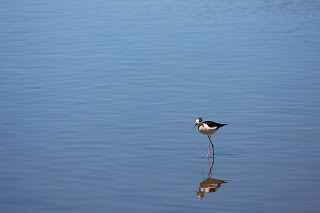
Photo of the Day - Black-Winged Stilt


Read more...

Thursday, March 3, 2011

Photo of the Day - In a Fish Bowl


Read more...

Wednesday, November 3, 2010

R tips - How to calculate diet indices from time-series data?

Ok, since I am supposed to write also about my work here, I'll start a new series called "R tips". R is an open source statistical program useful especially for nature scientists. This might be very nerdy and useless "shait" for the most, but I hope that some lucky Googlers find these tips useful. At least I have found this kind of blog entries very helpful when doing my work.

Lately I have been working with a seabird diet time-series. I have learned that there are tens of different indices that can be used to describe the dataset. Best fitting index has to be chosen individually depending on the questions and data. Swanson & Krapu (1974) made a review of the issue. Here I am going to demonstrate how to calculate "frequency of occurrence", "aggregate mass", "aggregate percentage" and mean mass for a time-series.

Shortly, frequency of occurrence tells how frequently a diet item occurs in the dataset. The aggregate mass tells the percentage for a diet item of summed total volume of all samples. Finally, the mean of mass percentages, or aggregate percentage, tells the average over the dataset of how many percentages a diet item constitutes of a stomach sample. This is much better explained in Swanson & Krapu 1974.

There are of course thousands of ways to do this, but simplest I have found so far is by using "reshape" package. Here is the R code:

#Assume a dataset where "a", "b" and "c" are diet items, "x1", "x2" ... are diet samples from individual birds and "y1" and "y2" are different years. Values for diet items are given in grams:

a <- c(1, 1, 2, 0, 3, 0, 5, 6, 1, 2)
b <- c(2, 1, 3, 2, 5, 2, 3, 5, 1, 0)
c <- c(0, 0, 1, 2, 4, 0, 20, 0, 0, 0)
year <- c(rep("y1", 5), rep("y2", 5))
bird <- paste(rep("x", 10), seq(1,10,1), sep="")

data <- cbind.data.frame(bird, year, a, b, c)

library(reshape)  # start the reshape package

data$total.mass <- rowSums(data[3:5]) # create total.mass column for later use
melt.data <- melt(data, id=1:2, measured=3:6) # melt the data so that we can cast it in desired format

# start from easiest, mean mass and standard deviation.

t(cast(melt.data, formula = year ~ variable, mean)) #Transposing t() because it is better to list diet items as rows when there are a lot of prey items
t(cast(melt.data, formula = year ~ variable, sd))

# aggregate mass needs column sum and total mass for each year

mass.sum <- cast(melt.data, formula = year ~ variable, sum)
aggregate.mass <- (mass.sum[2:5]/mass.sum$total.mass)*100

#if you want to print the dataframe, you can do following:

rownames(aggregate.mass) <- levels(mass.sum$year)
print(t(aggregate.mass), digits = 1)

#aggregate percentage

data.per <- cbind.data.frame(data[1:2], (data[3:6]/data$total.mass)*100) # calculate how big percentage each diet item consitutes in each sample
data.per <- data.per[-6] # drop off useless total.mass column
melt.data.per <- melt(data.per, id=1:2, measured=3:5)
aggregate.percentage <- cast(melt.data.per, formula = year ~ variable, mean)

#frequency of occurrence

data.na <- data
data.na[data.na==0] <- NA
melt.data.na <- melt(data.na, id=1:2, measured=3:6, na.rm = T)
occur <- cast(melt.data.na, formula = year ~ variable, length)
t(cbind.data.frame(occur[2:4]/occur$total.mass, row.names = levels(occur$year)))

#comparison between aggregate percentage and aggregate mass

rownames(aggregate.percentage) <- levels(aggregate.percentage$year)
aggregate.percentage <- aggregate.percentage[-1]
aggregate.mass <- aggregate.mass[-4]

aggregate.percentage-aggregate.mass

# differences are mainly because of 20 grams of item c in bird x7. The aggregate volume method gives equal weight to each unit of food consumed by any bird while the aggregate percent method gives equal weight in the analysis to each bird as Swanson & Krapu (1974) says.

Please tell, if there are mistakes in scripts.

References

Swanson, G. A., G. L. Krapu, et al. (1974). "Advantages in Mathematically Weighting Waterfowl Food-Habits Data." Journal of Wildlife Management 38(2): 302-307.

Read more...

Friday, September 24, 2010

Photos from the field season 2010


All my albums in Picasa are finally updated with fresh photos from field season 2010. You can check them out here.

Read more...

Thursday, September 23, 2010

Forskningsdagene


Forskningsdagene is a popular scientific event arranged once a year in Norway. The idea is that institutions are presenting their research for interested public. I think this is a great idea, since the public is often funding our research. Only problem with the event is that the "big names" are not having time to talk to the mortals. The task is often given for younger people. Well, on the other hand it's great fun for us and maybe we are as able to show scallops for kids as any experienced researcher...

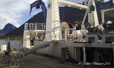
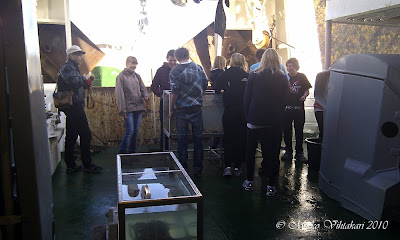
This was my second year with Forskningsdagene. My input for popular science this year was to take part for a cruise to Senjahopen with the University's research vessel Johan Ruud. This was also my first time, and probably the last for a long time, as a cruise leader. We went to show marine organisms for school kids on Senja. The science was not that interesting after all, but they found it incredibly entertaining when a sea cucumber was "pissing" on their pants...
Tomorrow we will anchor the boat to the harbour by Stortorget. The show starts at 11 o'clock. Come to check out where the sea cucumber pisses...

Read more...

Wednesday, September 22, 2010

No Health-Care for a Beaten Bird

In nature unexpected events follow each other. Many times observing nature is possible only, when you manage to forget observing yourself. Patience is the number one gift of a nature observer.
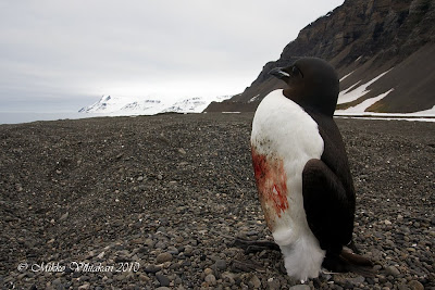
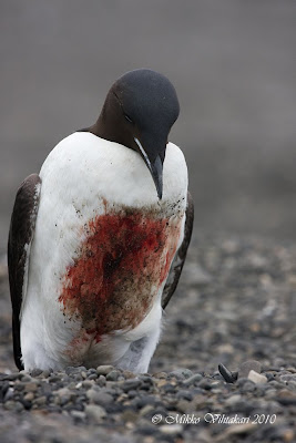
Guillemots seem to be a bird-world equivalent to people from India. The huge density of breeding colonies forces the birds to give an impression of compliant sitting next to each other, but real life in the colonies is often unlike the impression. Fights do occur. Fighting starts with slight pecking and sometimes develops into a serious attempt of murder. Most serious matches are solved in the air and finally end up into the ocean, where the weaker party is trying to escape by diving, flying, swimming and splashing from the murderous rage of the strong.
Sometimes Brünnich’s guillemots are bleeding after fighting, but I have never before seen any serious damage due to these fights. When counting birds in vicinity of tens of thousands of guillemots, probability of seeing rare occasions is higher. This combatant lost his fight and came to look for refuge from us, while swarming glaucous gulls were waiting to attack the beaten bird. There was not much we could do, except for taking photos. Finally we had to leave and the bird ended up as a meal for the hungry glaucous gulls. To live is to die. 

Read more...